It’s 2005 and the median U.S. income is $50,000. My client ‘Grow Smart’, a nonprofit, is looking to roll out a program nation wide in the U.S. to help people future plan. They want to help people under the current median income to achieve a median U.S. income and for people already above the median income grow into a better financial state. They will use my recommendations to look into and/or use key features in building their program for rollout.
I hypothesized that creating a classification model for ‘Grow Smart’ would allow them make accurate predictions on how to get people to the goal of making a median income and beyond. Using census data I built a classification model to make predictions on wether an individual would make above or below $50K.
After data acquisition, cleaning, EDA, and feature engineering I decided to use data from just the USA (90% of the data comes from the USA) and filtered for people working 40+ hors per week leaving me with 21K rows 21,378 rows / 44 columns to work with.
Tools Used:
Google Sheets, Pandas and Numpy for data acquisition, EDA, cleaning, and feature engineering
Imblearn for resampling unbalanced classes
Sklearn for modeling and parameter tuning
Grid Search for hyper-parameter optimization
Matplotlib and Seaborn for data and model visualization
4. EDA & Feature Engineering Workflow
After some initial EDA in Google Sheets the rest of the EDA and data cleaning was preformed in Python.
Starting with the Null values, they showed as ‘?’ in the dataset. They were treated as a missing value and replaced with NaN in the resulting DataFrame.
Some on the feature column names and cells had a space in the beginning (‘ age’) so it had to be stripped.
A few features were not going to be used so they were dropped.
At this point the dataframe looked like this.
Next I filtered for just the U.S. and people working 40+ hours per week.
I checked for Null values and dropped them.
prior shape:  (22174, 11)
post shape:  (21378, 11)
I wanted to more of an idea of all the data I was working with so I ran a loop to view all of the unique values in each feature.
Next I decided to rename some of the features.
It was necessary to change certain data into numerical data.
The rest of the non-numeric data was then changed to dummy variables for use in modeling. This changed my dataframe rows shape from 11 to 51 rows.
When the dummies were created it gave new columns for just the Null values in each feature, so they were dropped.
To prepare the data for modeling I had to drop the Target variable from the ‘X’ variable and I dropped ‘country_United-States’ since all the data in the dataframe is already filtered for the U.S.
A Target ‘y’ was then created for ‘income’.
5. Charts & Key Insights
In this section I created charts to help display interesting information that was found within the data set. I will go through each chart and explain what they show and how I interpret the information.
Note: Income is the target, 0 = (<=$50K) and 1 = (>$50K)
For the first chart I created a box plot to represent the relationship between age and income int he dataset.
The median age for a person making <=50K is 38 and the median for a person makeing >50K is 42.
What I gather from this is that the longer a person is in the workforce the more likely they are to make >50k. Most people who are in a carrer tend to move up in salary over time.
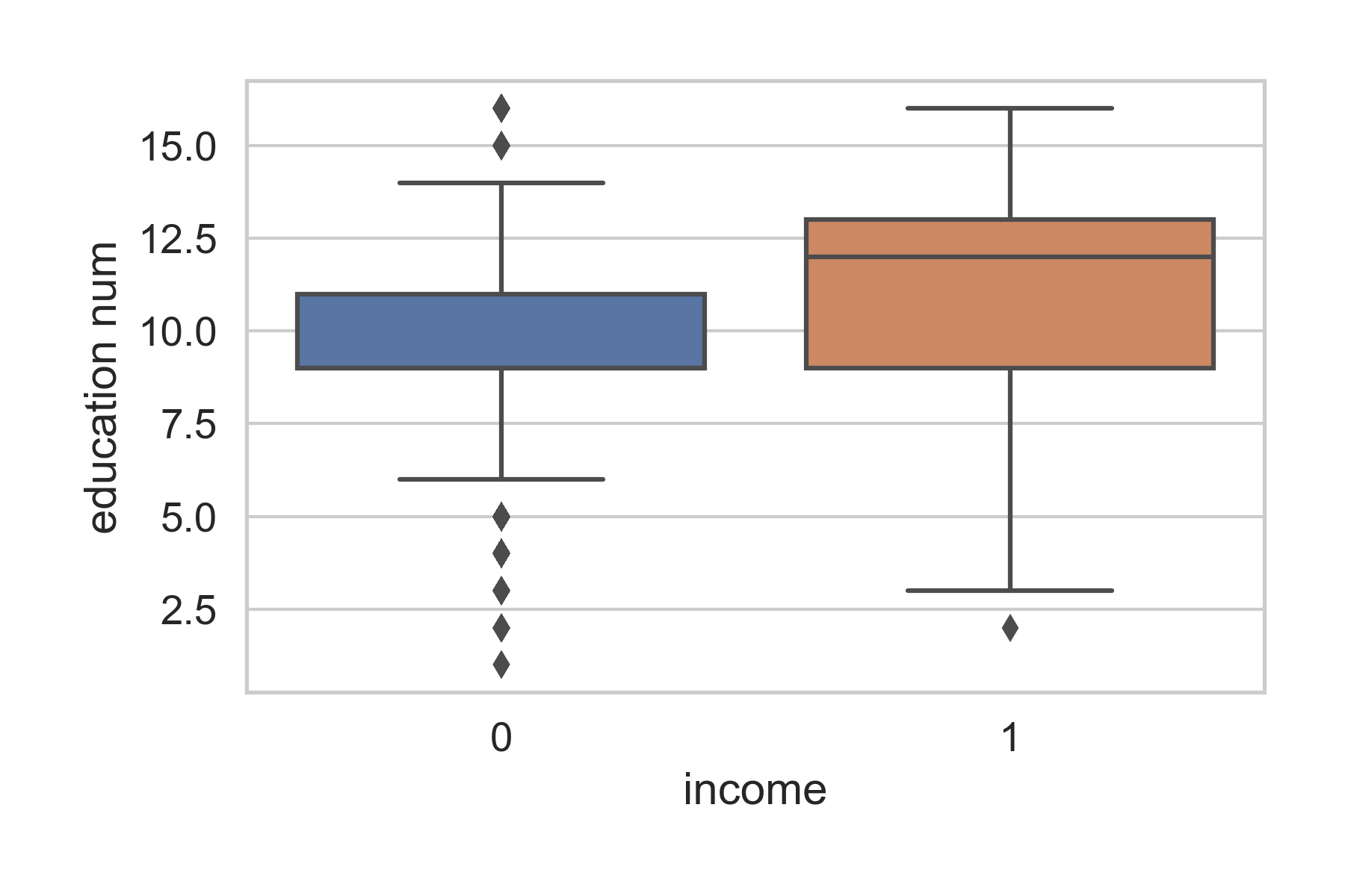
In the next box plot we see the relationship between education and income
People who have a median education level of ‘some college’ are more likely to make <=50k. People with a median education level of at least an associates degree are more likely to make >50k.
In the next chart we have a histogram of hours worked per week.
This shows that the majority of people working 40hrs per week make <=50k but even if a person works more than 40hrs they are not more likely to make >50k.
In his next chart we have a histogram of the connection between family relationship and income.
When it comes to family relationship the husban is the least likely to make <=50k and the most likely to make >50k. The situation is flipped for the wife. ‘Other Relative’ (nephew, grandparent, etc.) in this catigory, someone not making much or any income, is the most likley out of everyone to be making <=50k and least likely to be making >50k.
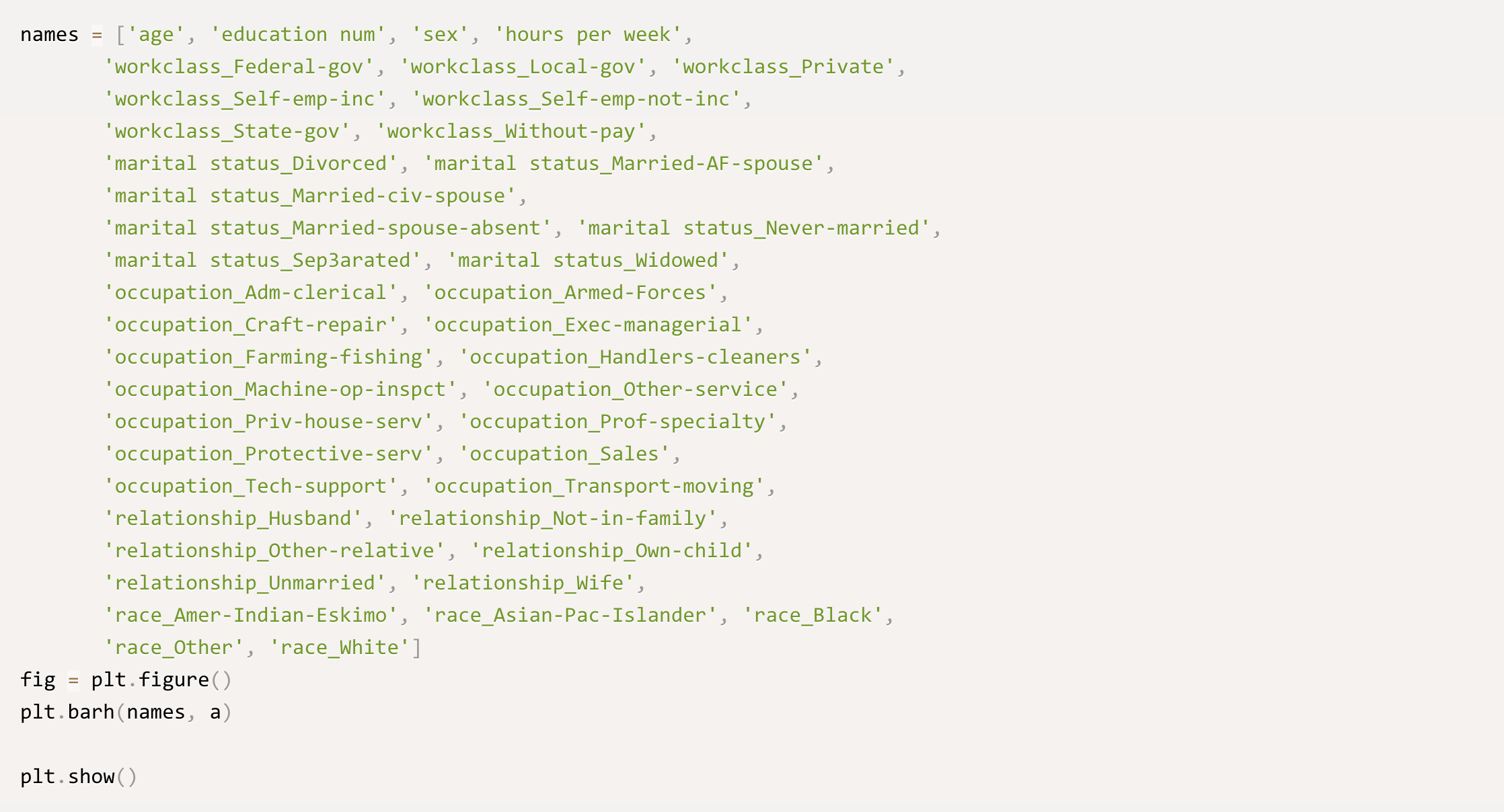
For the next chart we will take a look at the coefficient probabilities of all the features. I used the divide by 4 rule which will be explained after viewing the chart.
After feature engineering I was left with 43 features. Marked with the Red arrows are the standout coefficients. Below is a chart of their values.
I used the ‘divide by 4 rule’ to get my coefficients.
Interpretation using the ‘divide by 4 rule’: Using ‘Relationship- Wife’, a 1 unit increase (being a wife) will result in no more than a 32% positive difference in the probability that they will make >$50K.
All of the standout negative coefficients fall under ‘Marital Status’ (single people). What this is saying is that being single will decrease the the probability that one will make $50k by or up to 50%.
6. Modeling
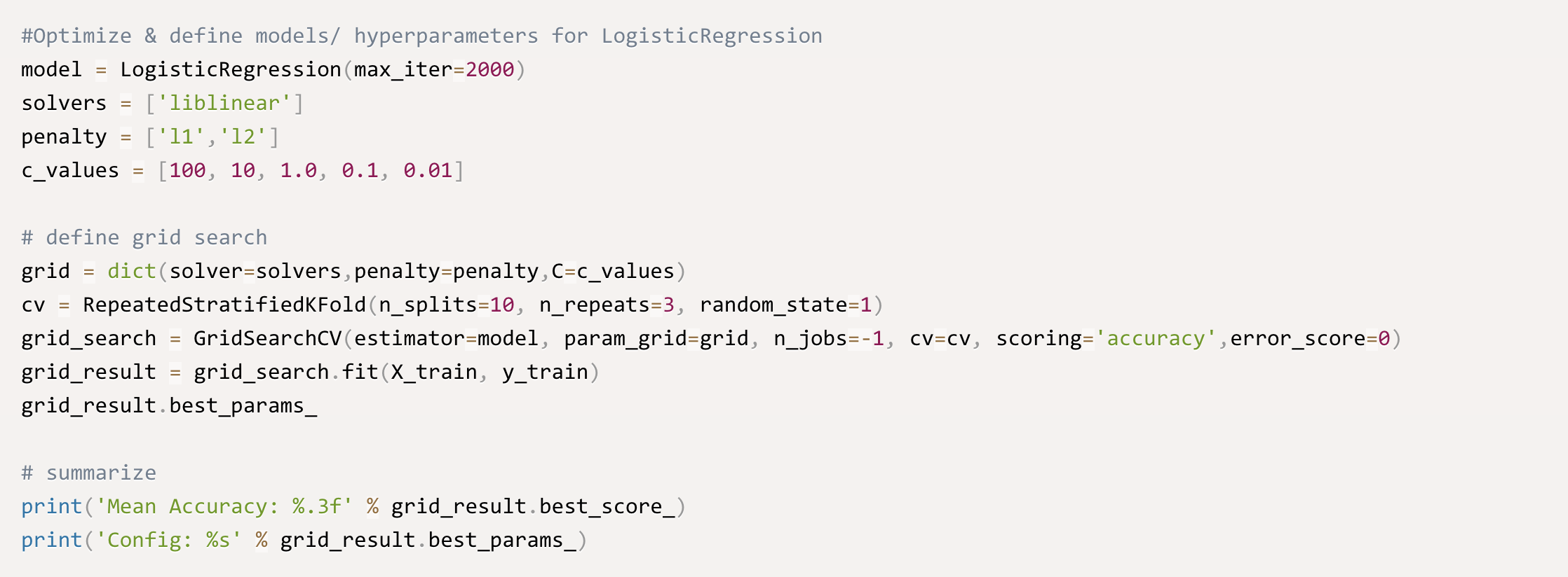
I implemented several different models for this project. The data was Scaled, grid search was used to optimize hyper-parameters for Logistic Regression and implemented a Train, Validate, Test Split: 60/20/20.
I will be showing code for one of the models the others are similar in setup.
Mean Accuracy: 0.803
Config: {'C': 1.0, 'penalty': 'l1', 'solver': 'liblinear'}